Alink漫谈(二十二) ：源码分析之聚类评估

0x00 摘要

Alink 是阿里巴巴基于实时计算引擎 Flink 研发的新一代机器学习算法平台，是业界首个同时支持批式算法、流式算法的机器学习平台。本文和上文将带领大家来分析Alink中 聚类评估 的实现。

0x01 背景概念

1.1 什么是聚类

聚类(Clustering)，用通俗的话来说，就是物以类聚，人以群分。

聚类是观察式学习，而不是示例式的学习。聚类能够作为一个独立的工具获得数据的分布状况，观察每一簇数据的特征，集中对特定的聚簇集合作进一步地分析。

聚类分析还可以作为其他数据挖掘任务（如分类、关联规则）的预处理步骤。

1.2 聚类分析的方法

聚类分析可以大致分为如下方法：

划分方法

• Construct various partitions and then evaluate them by some criterion,e.g.,minimizing the sum of square errors
• Typical methods:k-means,k-medoids,CLARANS

层次方法：

• Create a hierarchical decomposition of the set of data (or objects) using some criterion
• Typical methods: Diana,Agnes,BIRCH,CAMELEON

基于密度的方法：

• Based on connectivity and density functions
• Typical methods: DBSCAN,OPTICS,DenClue

基于网格的方法：

• Based on multiple-level granularity structure
• Typical methods: STING,WaveCluster,CLIQUE

基于模型的方法：

• A model is hypothesized for each of the clusters and tries to find the best fit of that model to each other
• Typical methods: EM,SOM,COBWEB

基于频繁模式的方法：

• Based on the analysis of frequent patterns
• Typical methods: p-Cluster

基于约束的方法：

• Clustering by considering user-specified or application-specific constraints
• Typical methods: COD(obstacles),constrained clustering

基于链接的方法：

• Objects are often linked together in various ways
• Massive links can be used to cluster objects: SimRank,LinkClus

1.3 聚类评估

聚类评估估计在数据集上进行聚类的可行性和被聚类方法产生的结果的质量。聚类评估主要包括：估计聚类趋势、确定数据集中的簇数、测定聚类质量。

估计聚类趋势：对于给定的数据集，评估该数据集是否存在非随机结构。盲目地在数据集上使用聚类方法将返回一些簇，所挖掘的簇可能是误导。数据集上的聚类分析是有意义的，仅当数据中存在非随机结构。

聚类趋势评估确定给定的数据集是否具有可以导致有意义的聚类的非随机结构。一个没有任何非随机结构的数据集，如数据空间中均匀分布的点，尽管聚类算法可以为该数据集返回簇，但这些簇是随机的，没有任何意义。聚类要求数据的非均匀分布。

测定聚类质量：在数据集上使用聚类方法之后，需要评估结果簇的质量。

具体有两类方法：外在方法和内在方法

• 外在方法：有监督的方法，需要基准数据。用一定的度量评判聚类结果与基准数据的符合程度。
• 内在方法：无监督的方法，无需基准数据。类内聚集程度和类间离散程度。

0x02 Alink支持的评估指标

Alink文档中如下：聚类评估是对聚类算法的预测结果进行效果评估，支持下列评估指标。但是实际从其测试代码中可以发现更多。

Compactness(CP), CP越低意味着类内聚类距离越近

\[\overline{CP_i}=\dfrac{1}{|C_i|}\sum_{x \in C_i}\|x_i-u_i\| \]

\[\overline{CP}=\dfrac{1}{k}\sum_{i=1}^{k}\overline{CP_k} \]

Seperation(SP),SP越高意味类间聚类距离越远

\[SP=\dfrac{2}{k^2-k}\sum_{i=1}^{k}\sum_{j=i+1}^{k}\|u_i-u_j\| \]

Davies-Bouldin Index(DB),DB越小意味着类内距离越小 同时类间距离越大

\[DB=\dfrac{1}{k}\sum_{i=1}^{k}max(\dfrac{\overline{CP_i}+\overline{CP_j}}{\|u_i-u_j\|}),i \not= j \]

Calinski-Harabasz Index(VRC),VRC越大意味着聚类质量越好

\[SSB=\sum_{i=1}^{k}n_i\|u_i-u\|^2 \]

\[SSW=\sum_{i=1}^{k}\sum_{x \in C_i}\|x_i-u_i\| \]

\[VRC=\dfrac{SSB}{SSW}*\dfrac{N-k}{k-1} \]

从其测试代码中，我们可以发现更多指标:

Assert.assertEquals(metrics.getCalinskiHarabaz(),12150.00,0.01);
Assert.assertEquals(metrics.getCompactness(),0.115,0.01);
Assert.assertEquals(metrics.getCount().intValue(),6);
Assert.assertEquals(metrics.getDaviesBouldin(),0.014,0.01);
Assert.assertEquals(metrics.getSeperation(),15.58,0.01);
Assert.assertEquals(metrics.getK().intValue(),2);
Assert.assertEquals(metrics.getSsb(),364.5,0.01);
Assert.assertEquals(metrics.getSsw(),0.119,0.01);
Assert.assertEquals(metrics.getPurity(),1.0,0.01);
Assert.assertEquals(metrics.getNmi(),0.01);
Assert.assertEquals(metrics.getAri(),0.01);
Assert.assertEquals(metrics.getRi(),0.01);
Assert.assertEquals(metrics.getSilhouetteCoefficient(),0.99,0.01);

我们需要介绍几个指标

2.1 轮廓系数（silhouette coefficient）：

对于D中的每个对象o，计算：

• a(o) : o与o所属的簇内其他对象之间的平均距离a(o) 。
• b(o) : 是o到不包含o的所有簇的最小平均距离。

得到轮廓系数定义为：

\[s(o)=\dfrac{b(o)-a(o)}{max\{a(o),b(o)\}} \]

轮廓系数的值在-1和1之间。

a(o)的值反映o所属的簇的紧凑性。该值越小，簇越紧凑。

b(o)的值捕获o与其他簇的分离程度。b(o)的值越大，o与其他簇越分离。

当o的轮廓系数值接近1时，包含o的簇是紧凑的，并且o远离其他簇，这是一种可取的情况。

当轮廓系数的值为负时，这意味在期望情况下，o距离其他簇的对象比距离与自己同在簇的对象更近，许多情况下，这很糟糕，应当避免。

2.2 Calinski-Harabaz（CH）

CH指标通过计算类中各点与类中心的距离平方和来度量类内的紧密度，通过计算各类中心点与数据集中心点距离平方和来度量数据集的分离度，CH指标由分离度与紧密度的比值得到。从而，CH越大代表着类自身越紧密，类与类之间越分散，即更优的聚类结果。

CH和轮廓系数适用于实际类别信息未知的情况。

2.3 Davies-Bouldin指数(Dbi)

戴维森堡丁指数(DBI)，又称为分类适确性指标，是由大卫L·戴维斯和唐纳德·Bouldin提出的一种评估聚类算法优劣的指标。

这个DBI就是计算类内距离之和与类外距离之比，来优化k值的选择，避免K-means算法中由于只计算目标函数Wn而导致局部最优的情况。

2.4 Rand index(兰德指数)(RI) 、Adjusted Rand index(调整兰德指数)(ARI)

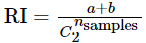
其中C表示实际类别信息，K表示聚类结果，a表示在C与K中都是同类别的元素对数，b表示在C与K中都是不同类别的元素对数。

RI取值范围为[0,1]，值越大意味着聚类结果与真实情况越吻合。RI越大表示聚类效果准确性越高 同时每个类内的纯度越高

为了实现“在聚类结果随机产生的情况下，指标应该接近零”，调整兰德系数（Adjusted rand index）被提出，它具有更高的区分度：

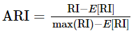
ARI取值范围为[−1,1]，值越大意味着聚类结果与真实情况越吻合。从广义的角度来讲，ARI衡量的是两个数据分布的吻合程度。

0x03 示例代码

聚类评估示例代码如下：

public class EvalClusterBatchOpExp {
    public static void main(String[] args) throws Exception {
        Row[] rows = new Row[] {
                Row.of(0,"0,0"),Row.of(0,"0.1,0.1,0.1"),"0.2,0.2,0.2"),Row.of(1,"9,9,9"),"9.1,9.1,9.1"),"9.2,9.2,9.2")
        };

        MemSourceBatchOp inOp = new MemSourceBatchOp(Arrays.asList(rows),new String[] {"label","Y"});

        KMeans train = new KMeans()
                .setVectorCol("Y")
                .setPredictionCol("pred")
                .setK(2);

        ClusterMetrics metrics = new EvalClusterBatchOp()
                .setPredictionCol("pred")
                .setVectorCol("Y")
                .setLabelCol("label")
                .linkFrom(train.fit(inOp).transform(inOp))
                .collectMetrics();

        System.out.println(metrics.getCalinskiHarabaz());
        System.out.println(metrics.getCompactness());
        System.out.println(metrics.getCount());
        System.out.println(metrics.getDaviesBouldin());
        System.out.println(metrics.getSeperation());
        System.out.println(metrics.getK());
        System.out.println(metrics.getSsb());
        System.out.println(metrics.getSsw());
        System.out.println(metrics.getPurity());
        System.out.println(metrics.getNmi());
        System.out.println(metrics.getAri());
        System.out.println(metrics.getRi());
        System.out.println(metrics.getSilhouetteCoefficient());
    }
}

输出为：

12150.000000000042
0.11547005383792497
6
0.014814814814814791
15.588457268119896
2
364.5
0.1199999999999996
1.0
1.0
1.0
1.0
0.9997530305375205

0x04 总体逻辑

代码整体逻辑如下：

• label 相关指标计算操作
  • 使用 calLocalPredResult 对每个分区操作
    • flatMap 1 是打散Row，得到 Label y
    • flatMap 2 是打散Row，得到 y_hat，所以前两步是得到 y 和 y_hat 的映射 map。这两个会广播给 CalLocalPredResult 使用。
    • 调用 CalLocalPredResult 建立混淆矩阵
  • 使用 reduce 归并这些分区操作结果。
  • 使用 extractParamsFromConfusionMatrix 根据混淆矩阵计算 purity,NMI等指标
• Vector相关指标计算操作
  • 对数据按照类别进行分组
  • 分组归并，调用 CalcClusterMetricsSummary分布式计算向量相关的指标
    • 遍历 rows，累积到 sumVector
    • 循环，计算出若干统计信息
  • 调用 ReduceBaseMetrics，再归并，形成一个BaseMetricsSummary
  • 调用 calSilhouetteCoefficient 来计算 SilhouetteCoefficient
  • 把数据存储为Params
• 合并输出
  • 做了一个 union，把 labelMetrics 和 vectorMetrics 联合起来，再归并输出到最后的表中
  • 分组归并
  • 输出到最后表

具体代码如下：

public EvalClusterBatchOp linkFrom(BatchOperator<?>... inputs) {
    BatchOperator in = checkAndGetFirst(inputs);
    String labelColName = this.getLabelCol();
    String predResultColName = this.getPredictionCol();
    String vectorColName = this.getVectorCol();
    DistanceType distanceType = getDistanceType();
    ContinuousDistance distance = distanceType.getFastDistance();

    DataSet<Params> empty = MLEnvironmentFactory.get(getMLEnvironmentId()).getExecutionEnvironment().fromElements(
        new Params());
    DataSet<Params> labelMetrics = empty,vectorMetrics;

    if (null != labelColName) { // 针对 label 操作
        // 获取数据
        DataSet<Row> data = in.select(new String[] {labelColName,predResultColName}).getDataSet();
        // 使用 calLocalPredResult 对每个分区操作
        labelMetrics = calLocalPredResult(data)
            .reduce(new ReduceFunction<LongMatrix>() { // 使用 reduce 归并这些分区操作结果
                @Override
                public LongMatrix reduce(LongMatrix value1,LongMatrix value2) {
                    value1.plusEqual(value2);
                    return value1;
                }
            })
            .map(new MapFunction<LongMatrix,Params>() { 
                @Override
                public Params map(LongMatrix value) {
                    // 使用  extractParamsFromConfusionMatrix 根据混淆矩阵计算 purity,NMI等指标
                    return ClusterEvaluationUtil.extractParamsFromConfusionMatrix(value);
                }
            });
    }
    if (null != vectorColName) {
        // 获取数据
        DataSet<Row> data = in.select(new String[] {predResultColName,vectorColName}).getDataSet();
      
        DataSet<BaseMetricsSummary> metricsSummary = data
            .groupBy(0) // 对数据按照类别进行分组
            .reduceGroup(new CalcClusterMetricsSummary(distance)) // 分布式计算向量相关的指标
            .reduce(new EvaluationUtil.ReduceBaseMetrics());// 归并
        DataSet<Tuple1<Double>> silhouetteCoefficient = data.map(  // 计算silhouette
            new RichMapFunction<Row,Tuple1<Double>>() {
                @Override
                public Tuple1<Double> map(Row value) {
                    List<BaseMetricsSummary> list = getRuntimeContext().getBroadcastVariable(METRICS_SUMMARY);
                    return ClusterEvaluationUtil.calSilhouetteCoefficient(value,(ClusterMetricsSummary)list.get(0));
                }
            }).withBroadcastSet(metricsSummary,METRICS_SUMMARY)
            .aggregate(Aggregations.SUM,0);

        // 把数据存储为Params
        vectorMetrics = metricsSummary.map(new ClusterEvaluationUtil.SaveDataAsParams()).withBroadcastSet( 
            silhouetteCoefficient,SILHOUETTE_COEFFICIENT);
    } else {
        vectorMetrics = in.select(predResultColName)
            .getDataSet()
            .reduceGroup(new BasicClusterParams());
    }

    DataSet<Row> out = labelMetrics
        .union(vectorMetrics) // 把 labelMetrics 和 vectorMetrics 联合起来
        .reduceGroup(new GroupReduceFunction<Params,Row>() { // 分组归并
            @Override
            public void reduce(Iterable<Params> values,Collector<Row> out) {
                Params params = new Params();
                for (Params p : values) {
                    params.merge(p);
                }
                out.collect(Row.of(params.toJson()));
            }
        });
    // 输出到最后表
    this.setOutputTable(DataSetConversionUtil.toTable(getMLEnvironmentId(),out,new TableSchema(new String[] {EVAL_RESULT},new TypeInformation[] {Types.STRING}) 
    ));
    return this;
}

0x05 针对 label 操作

5.1 calLocalPredResult

因为前面有 DataSet<Row> data = in.select(new String[] {labelColName,predResultColName}).getDataSet();，所以这里处理的就是 y 和 y_hat。

有两个 flatMap 串起来。

• flatMap 1 是打散Row，得到 Label y
• flatMap 2 是打散Row，得到 y_hat

两个 flatMap 都接了 DistinctLabelIndexMap 和 project(0)，DistinctLabelIndexMap 作用是 Give each label an ID,return a map of label and ID.，就是给每一个 ID 一个 label。project(0)就是提取出 label。

所以前两步是得到 y 和 y_hat 的映射 map。这两个会广播给 CalLocalPredResult 使用。

第三步是调用 CalLocalPredResult 建立混淆矩阵。

具体代码如下：

private static DataSet<LongMatrix> calLocalPredResult(DataSet<Row> data) {

    // 打散Row，得到 Label y
    DataSet<Tuple1<Map<String,Integer>>> labels = data.flatMap(new FlatMapFunction<Row,String>() {
        @Override
        public void flatMap(Row row,Collector<String> collector) {
            if (EvaluationUtil.checkRowFieldNotNull(row)) {
                collector.collect(row.getField(0).toString());
            }
        }
    }).reduceGroup(new EvaluationUtil.DistinctLabelIndexMap(false,null)).project(0);
    // 打散Row，得到 y_hat
    DataSet<Tuple1<Map<String,Integer>>> predictions = data.flatMap(new FlatMapFunction<Row,Collector<String> collector) {
            if (EvaluationUtil.checkRowFieldNotNull(row)) {
                collector.collect(row.getField(1).toString());
            }
        }
    }).reduceGroup(new EvaluationUtil.DistinctLabelIndexMap(false,null)).project(0);

    // 前两步是得到 y 和 y_hat 的映射 map。这两个会广播给 CalLocalPredResult 使用
    // Build the confusion matrix.
    DataSet<LongMatrix> statistics = data
        .rebalance()
        .mapPartition(new CalLocalPredResult())
        .withBroadcastSet(labels,LABELS)
        .withBroadcastSet(predictions,PREDICTIONS);

    return statistics;
}

CalLocalPredResult 建立混淆矩阵。

• open函数中，会从系统中获取 y 和 y_hat。
• mapPartition函数中，建立混淆矩阵。

matrix = {long[2][]@10707} 
 0 = {long[2]@10709} 
  0 = 0
  1 = 0
 1 = {long[2]@10710} 
  0 = 1
  1 = 0

代码是：

static class CalLocalPredResult extends RichMapPartitionFunction<Row,LongMatrix> {
    private Map<String,Integer> labels,predictions;

    @Override
    public void open(Configuration parameters) throws Exception {
        List<Tuple1<Map<String,Integer>>> list = getRuntimeContext().getBroadcastVariable(LABELS);
        this.labels = list.get(0).f0;
        list = getRuntimeContext().getBroadcastVariable(PREDICTIONS);
        this.predictions = list.get(0).f0;
    }

    @Override
    public void mapPartition(Iterable<Row> rows,Collector<LongMatrix> collector) {
        long[][] matrix = new long[predictions.size()][labels.size()];
        for (Row r : rows) {
            if (EvaluationUtil.checkRowFieldNotNull(r)) {
                int label = labels.get(r.getField(0).toString());
                int pred = predictions.get(r.getField(1).toString());
                matrix[pred][label] += 1;
            }
        }
        collector.collect(new LongMatrix(matrix));
    }
}

5.2 extractParamsFromConfusionMatrix

extractParamsFromConfusionMatrix 这里就是根据混淆矩阵计算 purity,NMI 等一系列指标。

public static Params extractParamsFromConfusionMatrix(LongMatrix longMatrix) {
    long[][] matrix = longMatrix.getMatrix();
    long[] actualLabel = longMatrix.getColSums();
    long[] predictLabel = longMatrix.getRowSums();
    long total = longMatrix.getTotal();

    double entropyActual = 0.0;
    double entropyPredict = 0.0;
    double mutualInfor = 0.0;
    double purity = 0.0;
    long tp = 0L;
    long tpFpSum = 0L;
    long tpFnSum = 0L;
    for (long anActualLabel : actualLabel) {
        entropyActual += entropy(anActualLabel,total);
        tpFpSum += combination(anActualLabel);
    }
    entropyActual /= -Math.log(2);
    for (long aPredictLabel : predictLabel) {
        entropyPredict += entropy(aPredictLabel,total);
        tpFnSum += combination(aPredictLabel);
    }
    entropyPredict /= -Math.log(2);
    for (int i = 0; i < matrix.length; i++) {
        long max = 0;
        for (int j = 0; j < matrix[0].length; j++) {
            max = Math.max(max,matrix[i][j]);
            mutualInfor += (0 == matrix[i][j] ? 0.0 :
                1.0 * matrix[i][j] / total * Math.log(1.0 * total * matrix[i][j] / predictLabel[i] / actualLabel[j]));
            tp += combination(matrix[i][j]);
        }
        purity += max;
    }
    purity /= total;
    mutualInfor /= Math.log(2);
    long fp = tpFpSum - tp;
    long fn = tpFnSum - tp;
    long totalCombination = combination(total);
    long tn = totalCombination - tp - fn - fp;
    double expectedIndex = 1.0 * tpFpSum * tpFnSum / totalCombination;
    double maxIndex = 1.0 * (tpFpSum + tpFnSum) / 2;
    double ri = 1.0 * (tp + tn) / (tp + tn + fp + fn);
    return new Params()
        .set(ClusterMetrics.NMI,2.0 * mutualInfor / (entropyActual + entropyPredict))
        .set(ClusterMetrics.PURITY,purity)
        .set(ClusterMetrics.RI,ri)
        .set(ClusterMetrics.ARI,(tp - expectedIndex) / (maxIndex - expectedIndex));
}

0x06 Vector相关

前两步是分布式计算 以及 归并：

DataSet<BaseMetricsSummary> metricsSummary = data
    .groupBy(0)
    .reduceGroup(new CalcClusterMetricsSummary(distance))
    .reduce(new EvaluationUtil.ReduceBaseMetrics());

6.1 CalcClusterMetricsSummary

调用了 ClusterEvaluationUtil.getClusterStatistics 来进行计算。

public static class CalcClusterMetricsSummary implements GroupReduceFunction<Row,BaseMetricsSummary> {
    private ContinuousDistance distance;

    public CalcClusterMetricsSummary(ContinuousDistance distance) {
        this.distance = distance;
    }

    @Override
    public void reduce(Iterable<Row> rows,Collector<BaseMetricsSummary> collector) {
        collector.collect(ClusterEvaluationUtil.getClusterStatistics(rows,distance));
    }
}

ClusterEvaluationUtil.getClusterStatistics如下

public static ClusterMetricsSummary getClusterStatistics(Iterable<Row> rows,ContinuousDistance distance) {
    List<Vector> list = new ArrayList<>();
    int total = 0;
    String clusterId;
    DenseVector sumVector;

    Iterator<Row> iterator = rows.iterator();
    Row row = null;
    while (iterator.hasNext() && !EvaluationUtil.checkRowFieldNotNull(row)) {
        // 取出第一个不为空的item
        row = iterator.next();
    }
    if (EvaluationUtil.checkRowFieldNotNull(row)) {
        clusterId = row.getField(0).toString(); // 取出 clusterId
        Vector vec = VectorUtil.getVector(row.getField(1)); // 取出 Vector
        sumVector = DenseVector.zeros(vec.size()); // 初始化
    } else {
        return null;
    }

    while (null != row) { // 遍历 rows，累积到 sumVector
        if (EvaluationUtil.checkRowFieldNotNull(row)) {
            Vector vec = VectorUtil.getVector(row.getField(1));
            list.add(vec);
            if (distance instanceof EuclideanDistance) {
                sumVector.plusEqual(vec);
            } else {
                vec.scaleEqual(1.0 / vec.normL2());
                sumVector.plusEqual(vec);
            }
            total++;
        }
        row = iterator.hasNext() ? iterator.next() : null;
    }

    DenseVector meanVector = sumVector.scale(1.0 / total); // 取mean

// runtime变量，这里示例是第二组的向量  
list = {ArrayList@10654}  size = 3
 0 = {DenseVector@10661} "9.0 9.0 9.0"
 1 = {DenseVector@10662} "9.1 9.1 9.1"
 2 = {DenseVector@10663} "9.2 9.2 9.2"  
  
    double distanceSum = 0.0;
    double distanceSquareSum = 0.0;
    double vectorNormL2Sum = 0.0;
    for (Vector vec : list) { // 循环，计算出几个统计信息
        double d = distance.calc(meanVector,vec);
        distanceSum += d;
        distanceSquareSum += d * d;
        vectorNormL2Sum += vec.normL2Square();
    }
  
// runtime变量
sumVector = {DenseVector@10656} "27.3 27.3 27.3"
meanVector = {DenseVector@10657} "9.1 9.1 9.1"
distanceSum = 0.34641016151377424
distanceSquareSum = 0.059999999999999575
vectorNormL2Sum = 745.3499999999999  
  
    return new ClusterMetricsSummary(clusterId,total,distanceSum / total,distanceSquareSum,vectorNormL2Sum,meanVector,distance);
}

6.2 ReduceBaseMetrics

这里是进行归并，形成一个BaseMetricsSummary。

/**
 * Merge the BaseMetrics calculated locally.
 */
public static class ReduceBaseMetrics implements ReduceFunction<BaseMetricsSummary> {
    @Override
    public BaseMetricsSummary reduce(BaseMetricsSummary t1,BaseMetricsSummary t2) throws Exception {
        return null == t1 ? t2 : t1.merge(t2);
    }
}

6.3 calSilhouetteCoefficient

第三步是调用 calSilhouetteCoefficient 来计算 SilhouetteCoefficient。

vectorMetrics = metricsSummary.map(new ClusterEvaluationUtil.SaveDataAsParams()).withBroadcastSet(
        silhouetteCoefficient,SILHOUETTE_COEFFICIENT);

这里就是和公式一样的处理

public static Tuple1<Double> calSilhouetteCoefficient(Row row,ClusterMetricsSummary clusterMetricsSummary) {
    if (!EvaluationUtil.checkRowFieldNotNull(row)) {
        return Tuple1.of(0.);
    }
    String clusterId = row.getField(0).toString();
    Vector vec = VectorUtil.getVector(row.getField(1));
    double currentClusterDissimilarity = 0.0;
    double neighboringClusterDissimilarity = Double.MAX_VALUE;
    if (clusterMetricsSummary.distance instanceof EuclideanDistance) {
        double normSquare = vec.normL2Square();
        for (int i = 0; i < clusterMetricsSummary.k; i++) {
            double dissimilarity = clusterMetricsSummary.clusterCnt.get(i) * normSquare
                - 2 * clusterMetricsSummary.clusterCnt.get(i) * MatVecOp.dot(vec,clusterMetricsSummary.meanVector.get(i)) + clusterMetricsSummary.vectorNormL2Sum.get(i);
            if (clusterId.equals(clusterMetricsSummary.clusterId.get(i))) {
                if (clusterMetricsSummary.clusterCnt.get(i) > 1) {
                    currentClusterDissimilarity = dissimilarity / (clusterMetricsSummary.clusterCnt.get(i) - 1);
                }
            } else {
                neighboringClusterDissimilarity = Math.min(neighboringClusterDissimilarity,dissimilarity / clusterMetricsSummary.clusterCnt.get(i));
            }
        }
    } else {
        for (int i = 0; i < clusterMetricsSummary.k; i++) {
            double dissimilarity = 1.0 - MatVecOp.dot(vec,clusterMetricsSummary.meanVector.get(i));
            if (clusterId.equals(clusterMetricsSummary.clusterId.get(i))) {
                if (clusterMetricsSummary.clusterCnt.get(i) > 1) {
                    currentClusterDissimilarity = dissimilarity * clusterMetricsSummary.clusterCnt.get(i) / (clusterMetricsSummary.clusterCnt.get(i) - 1);
                }
            } else {
                neighboringClusterDissimilarity = Math.min(neighboringClusterDissimilarity,dissimilarity);
            }
        }
    }
    return Tuple1.of(currentClusterDissimilarity < neighboringClusterDissimilarity ?
        1 - (currentClusterDissimilarity / neighboringClusterDissimilarity) :
        (neighboringClusterDissimilarity / currentClusterDissimilarity) - 1);
}

6.4 SaveDataAsParams

第四步是把数据存储为Params

public static class SaveDataAsParams extends RichMapFunction<BaseMetricsSummary,Params> {
    @Override
    public Params map(BaseMetricsSummary t) throws Exception {
        Params params = t.toMetrics().getParams();
        List<Tuple1<Double>> silhouetteCoefficient = getRuntimeContext().getBroadcastVariable(
            EvalClusterBatchOp.SILHOUETTE_COEFFICIENT);
        params.set(ClusterMetrics.SILHOUETTE_COEFFICIENT,silhouetteCoefficient.get(0).f0 / params.get(ClusterMetrics.COUNT));
        return params;
    }
}

0x06 合并输出

这一步做了一个 union，把 labelMetrics 和 vectorMetrics 联合起来，再归并输出到最后的表中。

DataSet<Row> out = labelMetrics
    .union(vectorMetrics)
    .reduceGroup(new GroupReduceFunction<Params,Row>() {
        @Override
        public void reduce(Iterable<Params> values,Collector<Row> out) {
            Params params = new Params();
            for (Params p : values) {
                params.merge(p);
            }
            out.collect(Row.of(params.toJson()));
        }
    });

this.setOutputTable(DataSetConversionUtil.toTable(getMLEnvironmentId(),new TypeInformation[] {Types.STRING})
));

0xFF 参考

聚类算法及其评估指标

[ML] 聚类评价指标

聚类结果的评价指标

聚类评价指标

如何评价聚类结果的好坏？

聚类评估算法-轮廓系数（Silhouette Coefficient ）

聚类效果好坏的评价指标

ARI聚类效果评价指标

聚类算法评价指标——Davies-Bouldin指数(Dbi)

【每周一博】浅说Davies-Bouldin指数（DBI）

聚类算法评价指标

聚类模型性能评价指标